DIRECTLY OBSERVED VARIABLES
DIME
Debiased causal analysis with Interactions for Mediation Estimation in ultra-high dimensions
Many measured variables, with a sparse structure in the regression coefficients.
Regularization and debiasing
Estimation and inference for direct and indirect effects with high-dimensional covariates and mediators.
TREATMENT → MEDIATOR → OUTCOME
SOFTWARE DEMONSTRATION
Load a simulation or your own CSV. Assign the variables, describe your measurements, and run an analysis with uncertainty and parameter sensitivity.
Click Load example in the Factor card.
Click Bulk assignment to review the suggested column groups.
Keep the suggested roles and click Confirm variables.
This example has complete data. Review overlap, then click Continue to analysis path.
Select Noisy measurements for this latent-factor example.
Click Linear factor. The app checks the dimensions of X and M.
Click Continue to settings.
Keep the 50% threshold. Click Variance & scree plot to inspect the selected factors.
Click the same heading to collapse the diagnostic.
Click the Bootstrap switch. Keep 20 completed refits for this short demonstration.
Click Sensitivity to latent dimensions to choose a comparison grid.
Click the mediator To field and enter 2: the M grid is 1–2.
Click the covariate From field and enter 2: the X grid is 2–3.
Check 20 bootstrap refits and four grid combinations, then click Run analysis.
20 bootstrap refits and all four sensitivity combinations completed.
Read the estimates and 95% bootstrap intervals. Download CSV exports these values.
Click NDE to compare the direct effect across factor dimensions.
Click View NDE grid values to expand the estimates behind the heatmap.
LOCAL INSTALLATION
Give the extracted kit to an AI assistant with access to your computer’s files and terminal. It can check your environment, install the dependencies, verify the R package and run the demo.
One kit includes the application, R package, example data, video and setup skill.
Open START-HERE.md and copy its request into a local coding assistant, such as Claude Code or Codex, with access to your files and terminal.
The checks run an R example and a real Factor analysis with bootstrap and sensitivity.
Download the complete workbench, install its dependencies once, and run analyses on your own computer. The download includes the browser interface, R analysis source, Python support and all five simulation datasets.
Save UHDmedi-local-workbench.zip, right-click the ZIP and choose Extract All. Open the extracted UHDmedi-local-workbench folder. Keep its files together; run the launchers from this folder, outside the ZIP.
1-Setup.cmdInstall dependencies once2-Start-Workbench.cmdStart the workbench whenever you need itapp/Website, analysis code and example CSVsLocal-user-guide.htmlThis illustrated guide, available offlinedocs/workbench-demo.mp4The video walkthrough, available offlineYou need a 64-bit installation of R for Windows and Python 3.11 or 3.12. If both are already installed, continue to the next step. For a new Python installation, enable Add python.exe to PATH. RStudio is optional.
The setup step needs an internet connection to download R packages and the Python libraries used by MediEncoder. It creates a project-specific environment inside the extracted folder.
Double-click 1-Setup.cmd and keep the setup window open until it finishes. This installs dependencies for Sparsity, Linear factor, MediEncoder and missing-data handling, and attempts to install the optional multiply robust method.
Read the final dependency check before closing the window. If the optional multiply robust dependencies are unavailable, the three main methods can still be used when their checks pass. The interface shows which methods are ready.
Double-click 2-Start-Workbench.cmd. Leave its window open while using the workbench. Open http://127.0.0.1:8765/ in your browser if it does not open automatically. The sidebar should report Local R service connected. On the first launch, dependency checks can take a minute; wait for this status before running an analysis.
Closing the server window stops the local website. Start it again with the same launcher next time. Opening index.html alone displays the interface without starting the analysis service.

This is the same synthetic example used in the video: 300 observations, 400 X measurements and 500 M measurements.
In the Factor card, click Load example. Roles are filled for you: outcome is Y, treatment is A, x_measure_* are X and m_measure_* are M. Leave sample_id ignored. Confirm that control is 0 and treated is 1, then click Confirm variables.
The example is complete, so keep Keep data unchanged. Review the treatment-assignment overlap plot, then click Continue to analysis path. Under What do you observe?, choose Noisy measurements, followed by Linear factor. Click Continue to settings.

Keep Cumulative explained variance at 50% and Center and standardize. The example selects two factors for X and two for M. Expand Variance & scree plot to inspect the choice.
Turn on Bootstrap Uncertainty and set Completed bootstrap replicates to 20 for this walkthrough. To include the video’s four-cell sensitivity grid, turn on Sensitivity to latent dimensions and use the ranges below.
| Setting | From | To | Step |
|---|---|---|---|
| Mediator dimensions | 1 | 2 | 1 |
| Covariate dimensions | 2 | 3 | 1 |
The grid refits four dimension pairs; your primary estimate still uses the two factor counts selected above. Click Run analysis and wait for Completed R analysis.

NIE is the natural indirect effect, NDE is the natural direct effect and TE is the total effect. Read their estimates and confidence intervals together. An interval containing zero does not establish that the effect is exactly zero.
In the sensitivity panel, switch among NIE, NDE and TE to see how the point estimates change with the dimension pair. This checks sensitivity to tuning choices, not to unmeasured confounding.
Choose Download CSV for the effect table and Download analysis record for the run configuration, results and diagnostics. Save them before starting a new session. If you change the inputs or settings, rerun the analysis to obtain results for the new configuration.

| Example | Your answer | Analysis path |
|---|---|---|
| Sparsity | Observed covariates and mediators | Sparsity; regularization applies to coefficients of X and M. |
| Factor | Noisy measurements | Choose Linear factor or MediEncoder. |
| Low-dimensional | Observed covariates and mediators | Multiply robust, when its optional dependencies are installed. |
| Sparsity · low-dimensional X | Observed covariates and mediators | Sparsity; coefficients of X remain unpenalized. |
| Factor · low-dimensional X | Noisy measurements | X remains observed; only M receives a factor representation. |
The last three examples are under More simulation datasets. For Sparsity, enable Sensitivity to balancing constants K₁ and K₂ to obtain a data-checked recommended range automatically. Adjust the two range bars if needed; the grid can contain at most 81 combinations per run. For factor methods, the variance slider offers 10%, 15%, …, 95%, 99%, and Eigenvalue ratio is an alternative dimension-selection rule.
Keep one observation per row and unique column names. Choose Choose CSV file, then assign one numeric Y, one binary A, numeric mediator columns M and baseline covariates X. X may contain categorical variables; the analysis service encodes them. Ignore identifiers and unrelated columns. Use Bulk assignment when there are many columns, and check the control/treated labels.
Choose a missing-data approach before continuing. Complete observations removes affected rows; mean/mode or median/mode fills them once; MICE multiple imputation creates several datasets and pools results. Simple imputation does not account for missing-value uncertainty. MICE with the factor methods requires bootstrap uncertainty.
Answer the measurement question based on your study. For observed variables, the app checks dimensions and routes to Sparsity or the multiply robust estimator. For noisy measurements, you choose Linear factor or MediEncoder. Low-dimensional X is retained directly. The treatment-overlap diagnostic is a useful data check; causal interpretation still requires the identification assumptions described in the papers.
The first image shows the extracted workbench running locally. The remaining images are from the recorded demonstration and use the same workflow and controls. Guide prepared October 4, 2026.
Run in your browser. The live application sends analysis data to the hosted R/Python service. Start with a simulation to explore the workflow.
Choose the scientific model. Users describe what their variables represent. The app checks dimensions; it cannot determine the causal assumptions from the data.
RESEARCH OVERVIEW
Causal mediation analysis studies how a treatment affects an outcome through intermediate variables. In high-dimensional data, those variables may be directly observed, or they may be latent processes measured through many noisy surrogates. This collection develops three approaches for these settings: sparse regression with multi-step debiasing, linear factor projections, and nonlinear representation learning. Each approach connects a structural model to estimation of a mediation functional and to statistical inference under explicit assumptions. The papers develop the theory, examine finite-sample behavior in simulations, and apply the methods to genomic studies of smoking, depression, and health outcomes. Mediation Workbench brings the analysis workflow into a browser, with examples, variable mapping, uncertainty estimates, and parameter sensitivity.
01 / METHODS
The methods target the same type of mediation functional under different measurement models. They differ in how they represent high-dimensional covariates and mediators.
DIRECTLY OBSERVED VARIABLES
Debiased causal analysis with Interactions for Mediation Estimation in ultra-high dimensions
Many measured variables, with a sparse structure in the regression coefficients.
NOISY MEASUREMENTS · LINEAR
Noisy measurements represent latent mediators, with observed or latent covariates.
NOISY MEASUREMENTS · NONLINEAR
Nonlinear encoder-decoder models for latent covariate and mediator representations.
| Modeling choice | DIME | FARMA | MediEncoder |
|---|---|---|---|
| What is measured? | Covariates and mediators directly | Noisy surrogates of latent variables | Noisy surrogates of latent variables |
| How is dimension handled? | Sparse regression coefficients | Linear factor projections | Learned nonlinear representations |
| Estimation strategy | Balancing and multi-step debiasing | Factor projection and cross-fitted regression | Coupled encoders and cross-fitted influence functions |
| Shared target | A mediation functional, with contrasts yielding natural direct and indirect effects | ||
For observed variables, the app routes to Sparsity when dim(X) + dim(M) > n, and to a low-dimensional multiply robust method otherwise. Low-dimensional X stays unpenalized in Sparsity and observed in the factor methods. These dimension checks do not determine whether your measurements are noisy or validate the modeling assumptions.
02 / CAUSAL MEDIATION
A treatment can change an outcome directly, or indirectly through a mediator. Causal mediation analysis separates these pathways to study how an effect arises.
For treatment a ∈ {0, 1} and mediator value m:
The observed outcome matches the corresponding potential outcome.
The observed mediator matches its potential value under the treatment received.
In the sparsity paper, for all relevant a, x, m and some uniform ε > 0:
Both treatment arms must be possible within each baseline stratum.
The mediator’s conditional density must be positive over the comparison’s support.
For a, a′ ∈ {0, 1} and mediator value m; ⫫ denotes conditional independence.
Given X, treatment and mediator are jointly independent of the potential outcome.
Given X, treatment is independent of the potential mediator.
Cross-world independence connects potential outcomes and mediators across treatment regimes.
Factor models: apply analogous assumptions to latent covariate and mediator factors. See FARMA and MediEncoder for their positivity and independence conditions.
FOLLOW THE PATHWAY
Note. Covariates and their arrows are omitted for clarity. M1, …, Mq are noisy measurements of the latent mediator factors fM; mediation operates through fM. Curved arrows indicate a nonlinear measurement map; their shapes are illustrative.
The total effect combines the direct effect and the effect transmitted through the mediator.
θ(a, a′) is a mean potential outcome. The effects below compare these means.
θ(a, a′) is a mean potential outcome. The effects below compare these means. fM(a′) denotes the latent mediator factors under treatment a′; observed M contains noisy measurements.
Select an effect to highlight its formula and pathway.
The mediator and outcome equations are linear, with coefficients that differ by treatment arm. Sparsity is imposed on the coefficients.
Eq. (2.3) · p. 6 ↗OUTCOME
MEDIATOR
B0 and B1 relate X to M. βa and γa are the outcome coefficients for X and M in arm a. The pairs (ϵ, ϵ′) and (U, U′) are centered random shocks.
The causal mechanism operates through latent factors. Both the latent structural equations and the mappings from factors to measurements are linear.
Eqs. (2.1)–(2.2) · p. 4 ↗LATENT MEDIATOR
OUTCOME
OBSERVED MEASUREMENTS
δa and αa are mediator and outcome intercepts. ΓX and ΓM are loading matrices. The structural noises uXM,0, uXM,1, ϵ0, ϵ1 and measurement errors uX, uM are centered.
Unknown functions describe the latent mediator and outcome mechanisms. The measurement maps from latent factors to X and M can also be nonlinear.
Eqs. (2.1)–(2.2) · p. 5 ↗LATENT MEDIATOR
OUTCOME
OBSERVED MEASUREMENTS
μ0∗ and μ1∗ are latent mediator functions; μ0 and μ1 are outcome functions. ϕX and ϕM are loading functions. The noise terms ϵ, ϵ′, uXM, u′XM, uX, and uM are centered.
Y(a,m) is the outcome under treatment a and mediator value m; M(a′) is the mediator under treatment a′. The mediator of interest is observed in the sparse model and latent in the surrogate models.
Identification requires consistency, treatment and mediator positivity, and the paper’s sequential-exchangeability and cross-world conditions. The factor and representation models also require informative measurements. Cross-fitting separates model fitting from effect evaluation. DIME distinguishes its sample-average target from the population target shown here, whose variance has an additional contribution.
A familiar example. An intervention may improve health partly by changing a biological process. Mediation asks how much of its effect operates through that process.
The high-dimensional challenge. We may observe many candidate mediators, or noisy measurements of a smaller latent system. Different measurement structures call for different methods.
03 / ESTIMATION
The procedures below summarize the estimation steps in each manuscript.
With many measured covariates and mediators, regularization stabilizes fitting but can introduce bias. The sparse method combines regression with balancing and multi-step correction.
FARMA projects noisy measurements into factor representations, fits treatment-specific regressions, and swaps folds before averaging. Under the factor-model assumptions, the identification error decreases as surrogate dimensions grow.
Coupled encoders learn nonlinear covariate and mediator representations. Separate data subsets handle training, tuning, nuisance estimation and final effect estimation.
04 / SIMULATIONS
Each tab reports a simulation setting from one paper, including RMSE, interval coverage, and distributional diagnostics where available.
The debiased estimator has lower RMSE than the plug-in estimator at four of the five reported sample sizes in this setting. At n = 250, the plug-in estimator has lower RMSE. The full curve shows both regimes.

| Sample size n | Debiased RMSE | Plug-in RMSE | 95% coverage¹ |
|---|---|---|---|
| 250 | 0.4450 | 0.2450 | 90.8% |
| 500 | 0.1750 | 0.3720 | 98.0% |
| 750 | 0.1680 | 0.3210 | 95.0% |
| 1,000 | 0.0970 | 0.2800 | 98.4% |
| 1,250 | 0.1040 | 0.2480 | 95.2% |
¹ Coverage for DIME; the analytical interval reported in the paper.
A separate low-noise setting makes the regularization bias visible. These distributions use the original 500 simulation draws for n = 750 and p + q = 1,500, with noise scale 0.1. The target is the fixed covariate-conditional mediation functional.
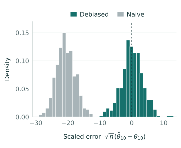
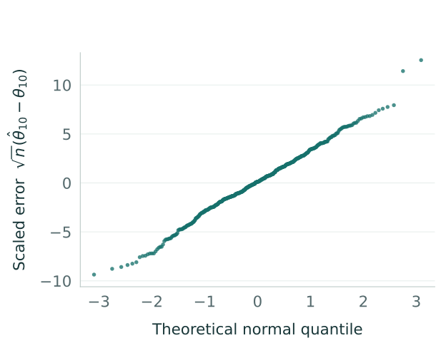
For this linear factor setting, RMSE decreases across the five sample sizes. Reported 95% interval coverage stays between 94.0% and 95.2%. These are finite-sample results for the stated factor model.

| Sample size n | FARMA RMSE | 95% coverage¹ |
|---|---|---|
| 500 | 0.2072 | 94.0% |
| 1,000 | 0.1350 | 95.2% |
| 1,500 | 0.1095 | 94.6% |
| 2,000 | 0.0945 | 95.2% |
| 2,500 | 0.0848 | 95.0% |
¹ Coverage for FARMA; the interval reported in the paper.
Under the nonlinear wavelet data-generating process, MediEncoder has the lowest RMSE among these four estimators at every reported sample size. The logarithmic vertical axis keeps both small- and large-sample behavior visible.

| Sample size n | MediEncoder RMSE | VAE RMSE | Autoencoder RMSE | Projection RMSE | 95% coverage¹ |
|---|---|---|---|---|---|
| 100 | 11.7200 | 47.0790 | 18.0240 | 31.0890 | 95.5% |
| 300 | 1.9310 | 2.2750 | 3.8590 | 9.1540 | 95.5% |
| 800 | 0.7660 | 0.8500 | 1.0530 | 1.0960 | 95.5% |
| 1,200 | 0.6610 | 0.7170 | 0.7640 | 0.7550 | 95.0% |
| 2,000 | 0.5130 | 0.5280 | 0.6230 | 0.5580 | 96.5% |
| 3,000 | 0.4700 | 0.4940 | 0.9260 | 0.5690 | 95.5% |
¹ Coverage for MediEncoder; the interval reported in the paper.
The papers use different data-generating processes and effect scales. Absolute RMSE values should be compared within a panel, rather than across the three papers.
05 / APPLICATIONS
The papers examine mediation in two genomic studies. The variable roles and the interpretation of the mediator differ across the analyses.
The sparse analysis treats methylation measurements as directly observed mediators. The outcome is log survival time in days.
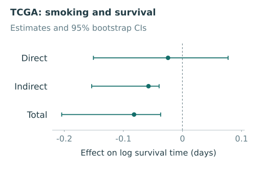
The reported indirect-effect interval is below zero, while the direct-effect interval includes zero. These estimates concern the joint methylation pathway under the study’s assumptions.
The factor analyses treat methylation as noisy measurements of latent mediators. The outcome is the original ADAS-Cog score.
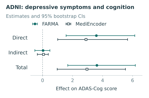
Both reported analyses have positive direct-effect estimates with intervals excluding zero. Their indirect-effect intervals include zero; the results do not establish a nonzero mediated effect in this application.
These are observational analyses under different structural models. Confidence intervals describe statistical uncertainty conditional on those assumptions; they do not by themselves establish a biological mechanism.
06 / PAPERS & CODE
Manuscripts and research implementations for DIME, FARMA, and MediEncoder.
Estimate mediation effects when covariates and mediators are directly observed but their dimensions can exceed the sample size. Sparse regressions, balancing weights, and multi-step debiasing accommodate treatment interactions while supporting inference.
@article{sparsity2024,
  title = {Debiased Causal Mediation Analysis in Ultra-High-Dimensional Settings in the Presence of Interaction Effects},
  author = {Bo, Shi and Ghassami, AmirEmad and Mukherjee, Debarghya},
  journal = {arXiv preprint arXiv:2412.08827},
  year = {2024},
  url = {https://arxiv.org/abs/2412.08827}
}Study mediation when the variables of interest are latent and observed only through many noisy surrogates. FARMA uses linear factor projections and cross-fitted regressions to estimate the mediation functional, with an identification approximation that improves as surrogate dimensions grow.
@article{farma2026,
  title = {Causal Mediation Analysis with High-Dimensional Surrogates: Identification, Estimation and Inference under Latent Factor Models},
  author = {Yadav, Himani and Bo, Shi and Ghassami, AmirEmad and Mukherjee, Debarghya},
  journal = {arXiv preprint arXiv:2611.03167},
  year = {2026},
  url = {https://arxiv.org/abs/2611.03167}
}Learn nonlinear covariate and mediator representations jointly from high-dimensional measurements. A coupled encoder-decoder architecture links treatment and covariate representations to the mediator representation, followed by cross-fitted influence-function estimation.
@article{mediencoder2026,
  title = {{MediEncoder}: Nonlinear Representation Learning for High-Dimensional Causal Mediation Analysis},
  author = {Bo, Shi and Mukherjee, Debarghya and Ghassami, AmirEmad},
  journal = {arXiv preprint arXiv:2606.30648},
  year = {2026},
  url = {https://arxiv.org/abs/2606.30648}
}